R Markdown
Sébastien Renaut (sebastien.renaut@gmail.com, Université de Montréal - QCBS)
March 20, 2019
Pre-requisite
Software
The latest version of R installed (R version 3.5.2).
 v.1.1 or better, Rstudio v.1.2 (Note that this version is not officially released yet).
- These packages need to be installed / updated:
install.packages("knitr")
install.packages("rmarkdown")
install.packages("rticles")
install.packages("tinytex")
tinytex::install_tinytex() #Please run this command as well to install a LaTeX distribution. This may take a few minutes to install (~150MB).Usefull trick: In Tools -> Global Options -> Code -> Display, check “Show whitespace characters”. This will let you see spaces and newlines characters in the editor.
Usefull trick: In Rstudio -> Preference -> Appearance. Change editor theme.
Course material
Workshop here: https://seb951.github.io/rmarkdown_workshop/Rmarkdown/rmarkdown_main.html
Download the workshop material on GitHub
 . Unzip and double-click on Rmarkdown.Proj file.

Don’t hesitate to comment (new issues) or request changes (pull request).
Follow the .html (web browser) and the .Rmd (R studio) documents. Try and experiment.
~2 hours: Introduction and practice
~10 minutes pause
~1 hour: other formats (.docx, .pdf and Shiny).
1 Introduction
Let’s look at a few examples on the Rstudio gallery
2 Markdown
Markdown is a lightweight markup language with plain text formatting syntax (Easy-to-read, easy-to-write plain text format). It is designed so that it can be easily converted to HTML and many other formats (e.g. PDF, MS Word, .docx).
Like other markup languages (e.g. HTML and Latex), it is completely independent from R.
Typically, files have the extension .md .
Look at this example. Examine the html render (GitHub automatically interprets .md files) and the raw file.

3 R Markdown
An extension of the Markdown syntax that enables R code to be embedded and executed.
Generate fully reproducible reports in different static and dynamic output formats.
Most of these packages are maintained by the R studio team (https://rmarkdown.rstudio.com/,
 Yihui Xie)
Plain text files that typically have the file extension .Rmd.
4 R Markdown basics

Write text & code in R studio.
Knit: The R package
rmarkdownfeeds the .Rmd file to the R packageknitr.knitrexecutes code and creates a new `Markdown (.md) document which includes the code and output.Subsequently tranformed into .html/.tex/.docx by
pandoc. (Note that .tex files need to be transformed bypdflatexinto .pdf files. We’ll come back to that later.)Pandocis an universal document converter, independent ofR.By default, R studio comes with
rmarkdown,knitr, andpandoc(but notpdflatex).When you click the Knit button (top left), a document will be generated that includes both content as well as the output of
Rcode within the document. You can also use therender()function.

4.1 Exercice 1: Setting up an R Markdown file
- This is easily done through R studio.

file > new file > R Markdown > HTML
Save it (“myfirstRmarkdown.Rmd”)
Knit
Examine the .html output.
Examine at the .Rmd file structure.
5 R Markdown syntax
Markdown provides an easy way to make standard types of formatted text, like:
italics (*text*) or italics (_text_)
bold (**bold**)
backslash (\) to interpret a special characters as character
“# and space” at the beginning of line for a header level (6 levels, # to ######)
bold italic (_**bold italic**_)
links (
[links](https://www.rmarkdown.rstudio.com))-
<!–comments–>
newline character: Two spaces and the end of line
paragraph mark: Two cariage returns
- list (first level using: * or + and space)
- item 1 (second level using: space, space, * or +, and space)
- item 2
- subitem 1a
- subitem 1b
- subsubitem 1b
- subitem 1a
- item 3
*** for an horizontal line
quoted text(`quoted text`)
> Quoted text: 1st way
> more quoted text
> still more quoted text
Quoted text: 1st way
more quoted text
still more quoted text
`Quoted text: 2nd way`
`more quoted text`
`still more quoted text`
Quoted text: 2nd way
more quoted text
still more quoted text
```
text: 3rd way
quoted text
more quoted text
```
Quoted text: 3rd way
more quoted text
still more quoted text - Tables
Species | Counts
——— | —–
H. sapiens | 24
M. musculus | 442
| Species | Counts |
|---|---|
| H. sapiens | 24 |
| M. musculus | 442 |
- The cheatsheet is your friend.
5.1 Exercice 2
Write some text now (add italicized/bold text, some URLs, and an itemized list, have fun!).
You can use this wikipedia text and list of roses subgenera as an example to reproduce.

Convert the document to a html webpage.
6 Header
---
title: "Rmarkdown"
author: "Sebastien Renaut"
date: '2018-03-12'
output: html_document
--- Header, metadata, YAML, YAML Ain’t Markup Language (https://en.wikipedia.org/wiki/YAML#History_and_name)
Header specifies configurations (what kind of document will be created, and the options chosen).
It is not required (defaults then apply).
It uses
Python-style indentation to specify some options.Many options possible depending what type of document you are generating. See below for some examples.
Note that some options can be specified either for the whole document (in the header), the code chunks, or both (chunks options supersede header). More on code chunks later.
6.1 Customizing header
---
title: "Rmarkdown"
author: "Sebastien Renaut"
date: "March 20, 2019"
output:
html_document:
code_folding: hide
highlight: tango
number_sections: T
theme: cerulean
toc: yes
toc_depth: 3
--- Note the indentation in the .Rmd document for the output options.
Note that date is populated via an
Rfunction.
6.2 Outputs
See the official R markdown lessons for more information. But these are some formats of interest:
output: html_documentoutput: ioslides_presentationoutput: pdf_document(This will require that you have a Latex software installed - We’ll get to that later).output: word_document(.docx)interactive
shinyapps (We’ll get to that later as well).
6.3 Table of content
toc: yesGenerate Table of Content.toc_depth:3depth of TOC.number_sections:TAdd section numbering to headers. Note that if you do not want a certain heading to be numbered, you can add{-}or{.unnumbered}after the heading, e.g.,
- More options in official R Markdown book.
6.4 Theme, highlight & other options
theme:specifies the theme to use for the page (“cerulean”, “journal”, “flatly”, “readable”, “spacelab”, “united”, and “cosmo”).highlight:Code syntax highlighting style (e.g. “tango”, “pygments”, “kate”, “zenburn”).code_folding: hideCode is hidden, but each chunk has it’s own button for showing or hiding code.See the cheatsheet and official R markdown book for more options.
6.5 Exercice 3
Change theme of your
R MarkdowndocumentChange highlighting
Add Table of Content
Save, knit and play with options.
7 Code chunks
The real power of
R Markdowncomes from mixingMarkdownsyntax with chunks of code.A code chunk is intepreted by
knitr. It works essentially the same as theRsyntax we are familiar with.A main code chunk may look like this:
```{r example, include = T, message = T, warning=T, echo = F, fig.cap="A figure of random points"}
#Running some R code.
x = rexp(1000)
min(x)
max(x)
hist(x)
``` ## [1] 0.0008266717## [1] 8.883759
A figure of random points
On the 1st line, I specify that I will run the
Rprogramming language.Then, I give the chunk a UNIQUE name and specify options.
There are a large number of chunk options in
knitrdocumented here.- Here are common options:
include = FALSE: Code and results will NOT appear in the finished file. Code is still interpreted, and the results can be used by other chunks.echo = Fprevents code, but not results from appearing in the finished file. This is a useful way to embed figures.message = Fprevents messages that are generated by code from appearing in the finished file.warning = Fprevents warnings that are generated by code from appearing in the finished file.fig.cap = "..."adds a caption to graphical results.fig.width=...,fig.height=...can also change figure width/heigth.
By default R studio creates a Global Options code chunk. Let’s examine this chunk:
```{r setup, include=FALSE}
knitr::opts_chunk$set(echo = TRUE)
``` see cheat sheet for more info.
Note that you can also run inline code. For example, ` r 10+5 ` would be processes as 15.
7.1 Exercice 4
- Add a code chunks that will:
- load an R package and make a plot
- load an R package and print some output of a function
- load an R package and make a plot
Run inline code.
Can you find options to print code, but not run it?
Also, try clicking the green arrow in the .Rmd on the right to execute a code chunk and preview its output.
7.2 More on code chunks
R Markdown can read and execute different languages!
## rmarkdown_main.Rmd
## rmarkdown_main.html
## rmarkdown_main.log## ['hello', 'python!']## Hello perl!8 Math symbols
Mathematical material is set off by the use of single dollar-sign characters (similar as in the LaTeX typesetting language).
So to write \(E = mc^{2}\), you’d write: $E = mc^{2}$
\(\sum_{i=1}^n ASV\)
\(F_{(1,69)}\) = 1.27, p-value=0.26
\(A = \pi*r^{2}\)
\(\sqrt{b^2 - 4ac}\)
If you need to use an actual dollar sign, you need to preface it with a back-slash \(E = mc^{2}\) versus $E = mc^{2}$
The use of double dollars quotations allows for displayed formulas (centered). \[\sqrt{b^2 - 4ac}\]
See more example equations from this McGill math R Markdown tutorial.
9 Include pictures & figures
There are several ways to include figures.
URL
Can be included from an URL directly uploaded from the web:
{width=250px}

Inline figure
If this figure is small, it can be added to the text directly: eg.: Today, we are using ![]() to generate webpages with
to generate webpages with ![]() images…
images…
Previously saved
This is an image previously saved in the figures directory
{width=250px}

In all these cases, graphs are rendered with pandoc and not knitr, so pandoc options need to be specified, not knitr R graphics options:
It’s simple, but options can be tricky.
You may need to play with spacing, figure size, and figure position.
Options are specified directly after the URL or link (eg. {width=250px} or {width=50%}).
knitr
Images can also be interpreted by knitr as below:
```{r graphic_example, out.width = "20%", fig.cap = "rosa_banksiae", echo = F,fig.align = "center"}
knitr::include_graphics("../figures/rosa_banksiae.JPG")
```rosa_banksiae
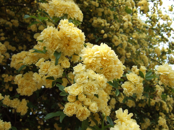
Wrapping text
```{r roses, out.width = "50%",echo = F,out.extra='style="float:right; padding:10px"'}
knitr::include_graphics("../figures/rosa_banksiae.JPG")
```
Subgenera and sections
The genus Rosa is subdivided into four subgenera:
- Hulthemia (formerly Simplicifoliae, meaning “with single leaves”) containing one or two species from southwest Asia, R. persica and R.berberifolia (syn. R. persica var. berberifolia) which are the only roses without compound leaves or stipules.
- Hesperrhodos (from the Greek for “western rose”) has two species, both from southwestern North America. These are R. minutifolia and R. stellata.
- Platyrhodon (from the Greek for “flaky rose”, referring to flaky bark) with one species from east Asia, R. roxburghii.
- Rosa (the type subgenus) containing
R generated
Graphs can also be generated directly by R code, specified in a code chunk (R options specified in the code chunk) and interpreted by knitr as we did previously.
```{r another example, echo = F, message = F}
library(ggplot2)
mtcars_ggplot = ggplot(mtcars, aes(x=wt, y=mpg)) +
geom_point() + geom_smooth()
mtcars_ggplot
```
Two figures in two columns
```{r out.width=c('50%', '50%'), fig.show='hold',echo=F,message = F}
mtcars_ggplot
plot(rnorm(10))
```## `geom_smooth()` using method = 'loess' and formula 'y ~ x'
10 Including Tables
By default, R Markdown displays data frames and matrices as they would be in the R terminal.

You can use the
knitr::kablefunction for additional formatting, as in the .Rmd file below.
## mpg cyl disp hp drat wt qsec vs am gear carb
## Mazda RX4 21.0 6 160 110 3.90 2.620 16.46 0 1 4 4
## Mazda RX4 Wag 21.0 6 160 110 3.90 2.875 17.02 0 1 4 4
## Datsun 710 22.8 4 108 93 3.85 2.320 18.61 1 1 4 1
## Hornet 4 Drive 21.4 6 258 110 3.08 3.215 19.44 1 0 3 1
## Hornet Sportabout 18.7 8 360 175 3.15 3.440 17.02 0 0 3 2
## Valiant 18.1 6 225 105 2.76 3.460 20.22 1 0 3 1#With kable function from knitr (better looking)
knitr::kable(head(mtcars),digits =1,caption = "A motorcars table")| mpg | cyl | disp | hp | drat | wt | qsec | vs | am | gear | carb | |
|---|---|---|---|---|---|---|---|---|---|---|---|
| Mazda RX4 | 21.0 | 6 | 160 | 110 | 3.9 | 2.6 | 16.5 | 0 | 1 | 4 | 4 |
| Mazda RX4 Wag | 21.0 | 6 | 160 | 110 | 3.9 | 2.9 | 17.0 | 0 | 1 | 4 | 4 |
| Datsun 710 | 22.8 | 4 | 108 | 93 | 3.8 | 2.3 | 18.6 | 1 | 1 | 4 | 1 |
| Hornet 4 Drive | 21.4 | 6 | 258 | 110 | 3.1 | 3.2 | 19.4 | 1 | 0 | 3 | 1 |
| Hornet Sportabout | 18.7 | 8 | 360 | 175 | 3.1 | 3.4 | 17.0 | 0 | 0 | 3 | 2 |
| Valiant | 18.1 | 6 | 225 | 105 | 2.8 | 3.5 | 20.2 | 1 | 0 | 3 | 1 |
10.1 Exercice 5
Find a picture on the web. Save it.
Add it to document either directly, or in a code chunk.
Try adjusting size.
Add a table using
knitr.
11 References
11.1 Footnotes
- Footnotes are easy when you have a few references1. Use
[^1]in text, and add reference at the end using this format:[^1]: Renaut 2019. R Markdown footnote. Number 1. pp1-2.
11.2 Bibliography
- Otherwise, you may specify a bibliography and citation style by adding these two lines in the header.
csl: ../csl/peerj.csl
bibliography: ../biblio/test_library.bib - Note that you may need to specify the file path or add them to the current directory.
Citation Style Language
The Citation Style Language (.csl) file specifies the reference format.
It is an open XML-based language that describe the formatting of citations and bibliographies. Reference management programs using .csl include Zotero, Mendeley and Papers3.
Most journals should have a .csl file be on this GitHub repo. But you could also create your own.
Bibliographic information
- A .bib file contains the bibliographic information of your document in bibTeX format (other formats possible).
@article{altschul1997gapped,
title={Gapped BLAST and PSI-BLAST: a new generation of protein database search programs},
author={Altschul, Stephen F and Madden, Thomas L and Sch{\"a}ffer, Alejandro A and Zhang, Jinghui and Zhang, Zheng and Miller, Webb and Lipman, David J},
journal={Nucleic acids research},
volume={25},
number={17},
pages={3389--3402},
year={1997},
publisher={Oxford University Press}
}Here, I created a .bib file (../biblio/test_library.bib) in the reference management software Papers3.
I often copy .bib references directly from Google Scholar and add it to a .bib database text file.

11.3 Citations
The bioinformatics program BLAST (Altschul et al., 1997) has been cited nearly 70,000 times. These are three random references (Thibert-Plante & Hendry, 2010; Wagner et al., 2012; Yoshida et al., 2014) from my database.
Each citation must have a unique key, composed of ‘@’ + the citation identifier from the .bib database file.
Citations go inside square brackets [ ] and are separated by semicolons (;).
You can also write in-text citations by removing the square brackets. For example, Altschul et al. (1997) is cited a lot.
A minus sign (-) before the @ will suppress mention of the author in the citation. This can be useful when the author is already mentioned in the text. For example, The BLAST algorithm by Stephen Altschul and a bunch of other people (1997) have been cited 70,000 times.
By default, references are added at the end of document. Use the code
<div id="refs"></div>to place references elsewhere.
11.4 Exercice 6
Find 3 papers in Google Scholar. Copy references to a text file (in bibTeX format). Save it with a .bib extension.
Find another Citation Style Language from this GitHub repo (e.g. Nature, PLOS ONE, Indian Journal Of Dermatology, etc.). (hint: type ‘t’ in GitHub repo to activate search function). Save as text file (.csl extension) and modify it in the header.
12 Cheatsheets and help
13 References
(Note that references below are generated automatically, except for the footnote.)
Altschul SF., Madden TL., Schäffer AA., Zhang J., Zhang Z., Miller W., Lipman DJ. 1997. Gapped blast and psi-blast: A new generation of protein database search programs. Nucleic acids research 25:3389–3402.
Thibert-Plante X., Hendry A. 2010. The consequences of phenotypic plasticity for ecological speciation. Journal Of Evolutionary Biology:1–17.
Wagner CE., Keller I., Wittwer S., Selz OM., Mwaiko S., Greuter L., Sivasundar A., Seehausen O. 2012. Genome-wide RAD sequence data provide unprecedented resolution of species boundaries and relationships in the Lake Victoria cichlid adaptive radiation. 22:787–798.
Yoshida K., Makino T., Yamaguchi K., Shigenobu S., Hasebe M., Kawata M., Kume M., Mori S., Peichel CL., Toyoda A., Fujiyama A., Kitano J. 2014. Sex Chromosome Turnover Contributes to Genomic Divergence between Incipient Stickleback Species. PLoS Genetics 10:e1004223.
Renaut 2019. R Markdown footnote. Number 1. pp1-2↩